Analysis of terrestrial laser scanning data for Landers 1992 earthquake fault scarp

by Ramón Arrowsmith, School of Earth and Space Exploration, Arizona State University

We (UT Dallas team and me) scanned the fault scarp that formed in the 1992 Landers earthquake in the Mojave Desert California in May 2008. This is a site that Dallas Rhodes and I have studied since immediately after the earthquake (see Arrowsmith and Rhodes, 1994 and Arrowsmith and Rhodes, 200?). Here is a link to some of other pictures from the site.

Here is an AGU 2009 presentation which includes analysis of these data: AGU09Arrowsmith_TLS.ppt

Data overview

We used the UTD Riegl terrestrial laser scanner. The data were processed by the UTD team. They gave me a 9.54 million point 3 column file of the laser returns that looks like this:

E,N,Z
540969.011,3822032.969,890.643
540969.011,3822032.97,890.643
540969.092,3822032.91,890.633
540970.323,3822032.053,890.932
540970.405,3822031.995,890.942
540970.487,3822031.938,890.952
540970.569,3822031.88,890.962

Here are the data to download in compressed ascii format: Combptcloud_LF.zip

Figure 1 shows an overview of the site and figures 2-4 zoom to the channels the changes in which we have monitored erosional change since 1992. Note that in the areas of high shot density in the areas of the channels, the 10 cm DEMs are very nice and show the channel landforms well. However, in the areas of lower shot density, the resulting DEM exhibits corduroy which is probably an artifact of the IDW local binning algorithm, rather than a stitching artifact. I am working on high performance interpolation tools which will hopefully fix this problem.

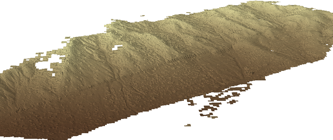
Figure 1. View of a hillshade made from the optimal DEM (0.1 resolution and 0.5 m search radius; see below). Color overlay shows illustrates shots per square meter. Note the channels that we emphasized have more than 33,000 shots per square meter (4 orders of magnitude more than a typical airborne laser scan!).

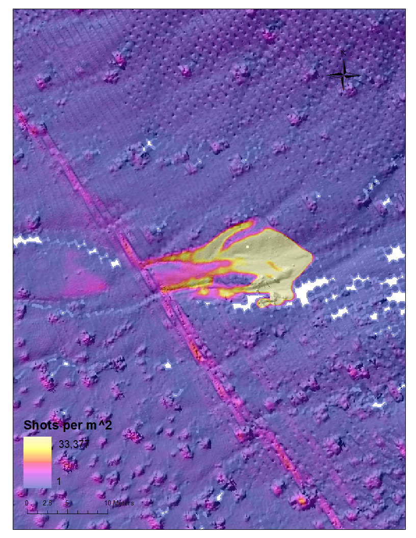Figure 2. NW channel zoom. Look here for a balloon photo of the site from 1998 of the site.

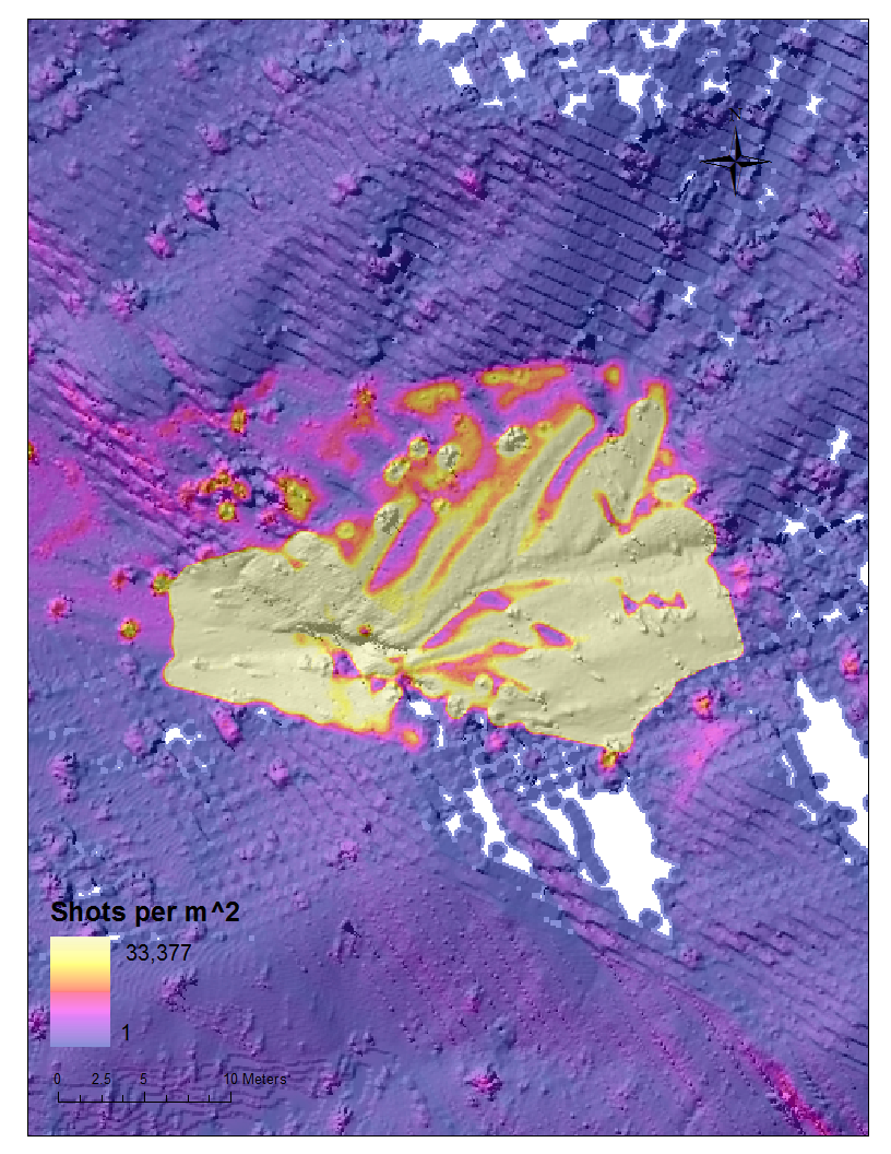
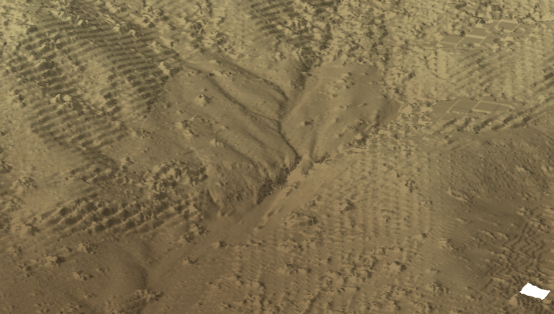Figure 3. Center channel zoom. Look here for a balloon photo of the site from 1998 of the site.

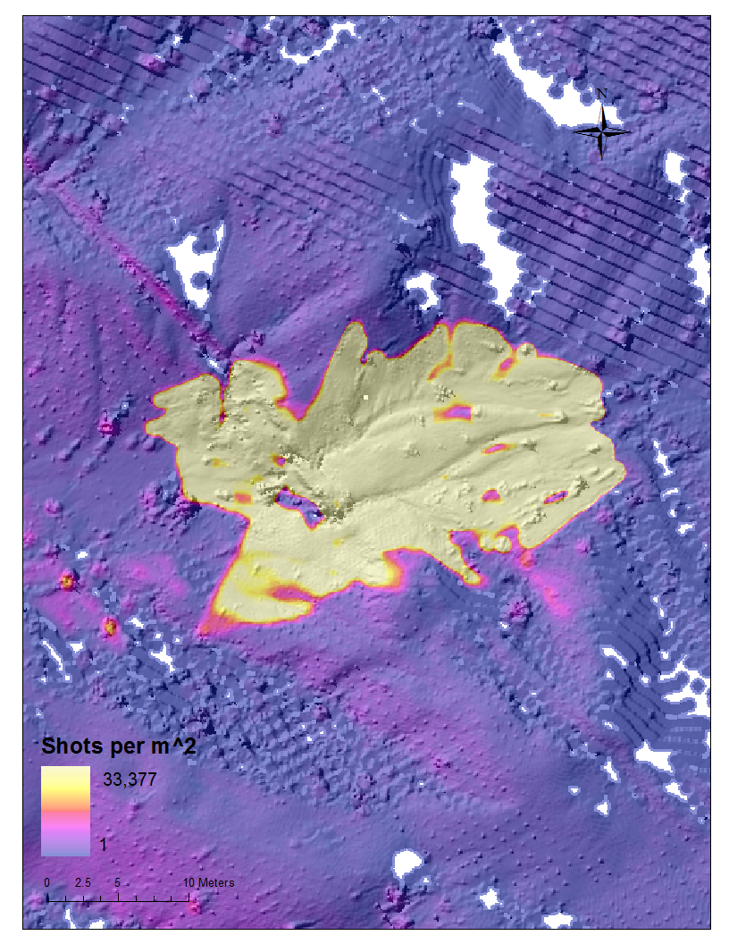
Figure 4. SE channel zoom.

Analysis of shot density and optimal DEM local binning search radius

The problem we faced was to analyze the data with the standard digital elevation model processing tools which we use for analysis of airborne laser scanning data and also for the geomorphic investigations typical for DEMs.

For those analyses, I have found that the inverse distance weighted local binning approach (see links here) works fairly well. In this simple DEM processing algorithm, the DEM grid node is estimated by computing the inverse distance weighted (1/r²) mean of the points within a specified search radius. If there are no points, a null value is assigned. The tradeoff comes then from having a large enough search radius to find at least one point for the grid node, and not using a point so far away from the grid node as to provide an unacceptable representation of the elevation. For a given DEM grid spacing, one can compute DEMs with progressively increasing search radii, and compute the number of nodes versus search radius. This will plot as a negatively sloping curve which becomes asymptotic to some finite number of nulls. An inflection point can be qualitatively determined, and that provides the optimal minimum search radius with the maximum number of acceptable nulls (Figure 5). For this dataset and a 0.1 m DEM, the optimal search radius is about 0.5 m.

Figure 5. # nulls versus search radius in meters. Optimal search radius is about 0.5 m for this 0.1 m DEM analysis.

Figures 6-8 show the effect of varying search radius on the resulting hillshade of a 0.1 m DEM. With a search radius of 0.1 m (Figure 2), much of the scene is null. The lower portion (to the west) was illuminated more easily from the station locations on the west side of the study area. The upper parts of the watershed were not scanned densely.

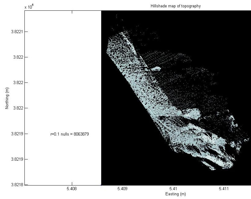
Figure 6. Hillshade map of 0.1 m DEM topography with 0.1 m search radius.

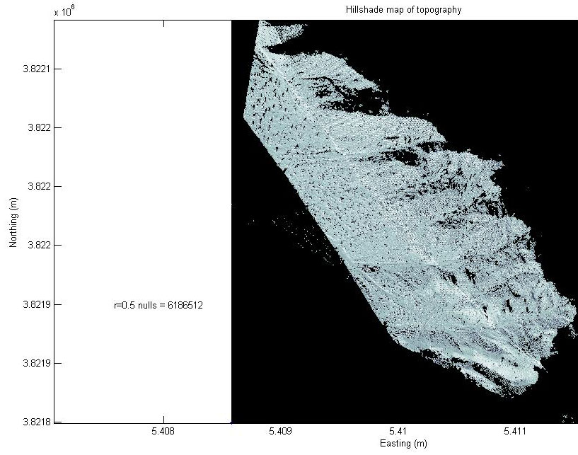
Figure 7. Hillshade map of 0.1 m DEM topography with 0.5 m search radius. This is optimal.

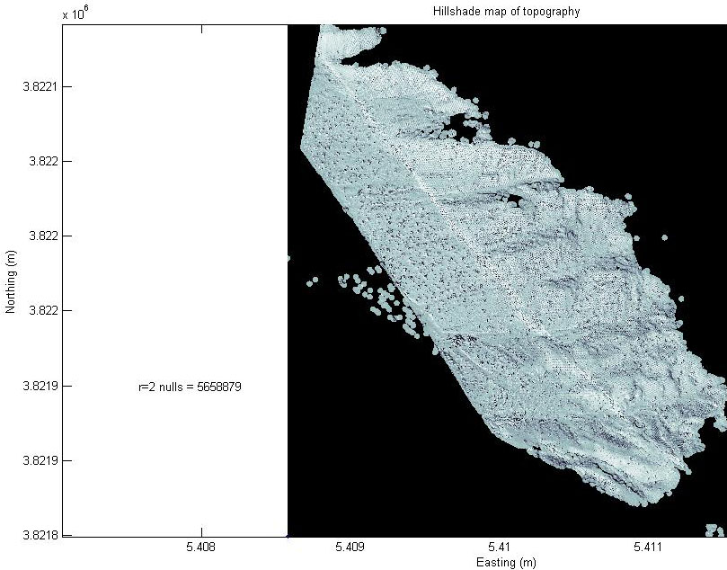
Figure 8. Hillshade map of 0.1 m DEM topography with 2 m search radius.

The 2 m search radius (Figure 8) covers a lot of ground, but probably is not representing the topography acceptably, so now, we can take the optimal 0.1 m DEM (Figures 1 and 7) and combine it with a broader DEM (2 m with a 2 m search radius; Figure 8) to make a blended DEM?

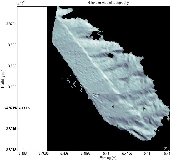
Figure 9. Hillshade map of 2 m DEM topography with 2 m search radius to be used as a background filler for the finer 0.1 optimal DEM.

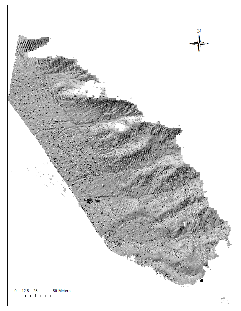
Figure 10. Hillshade map of 2 m DEM topography with 2 m search radius underneath the finer 0.1 optimal DEM.

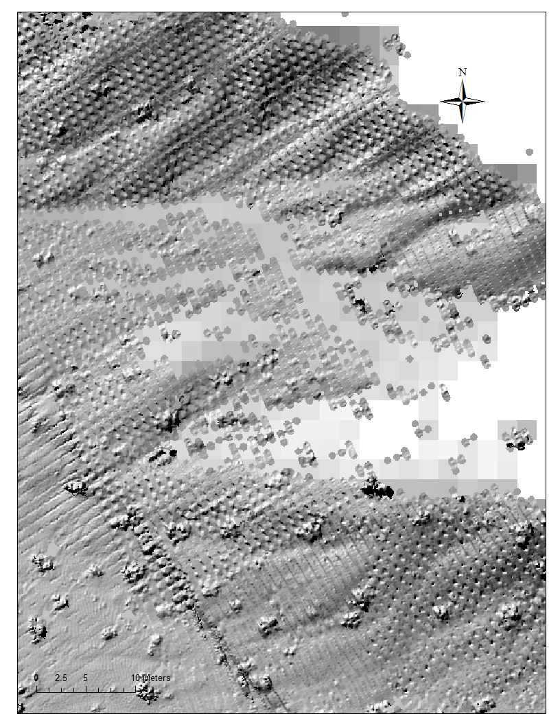
Figure 11. Hillshade map of 2 m DEM topography with 2 m search radius underneath the finer 0.1 optimal DEM zoomed to show combination.

Map algebra to compute a composite DEM

Given all of the individual analyses from above, is it possible to make a composite DEM, taking advantage of the increasing shot density towards the core of the survey?
I did this Spatial Analyst in ArcMap, with the options set as cell size (same as finest resolution DEM; 0.1 m in this case). My basic logic was to build a series of grids of the elevations (at the same resolution), starting with the interior resolved portion with the 0.5 m search radius, then take the 2 m DEM computed with the 2 m search radius and use its values where the 0.1 m DEM was null. Then add in the 5 m DEM computed with the 5 m radius beyond where the 2 m DEM was null. In Spatial Analyst--Raster Calculator these are the commands:
twombandb=IsNull([idwpt1pt5]) & [idw2_2] > 0
fivembandb=IsNull([idw2_2]) & [idw5_5] > 0
Zero out the base dem where null:
pt1pt5z = con(IsNull([idwpt1pt5]),0,[idwpt1pt5])

add together newpt1dem=[pt1pt5z] + [twombandb] * [idw2_2] + [fivembandb] * [idw5_5]

idwpt1p5 is the 0.1 m DEM with 0.5 m search radius.
idw2_2 is the 2 m DEM with the 2 m search radius.
idw5_5 is the 5 m DEM with the 5 m search radius.

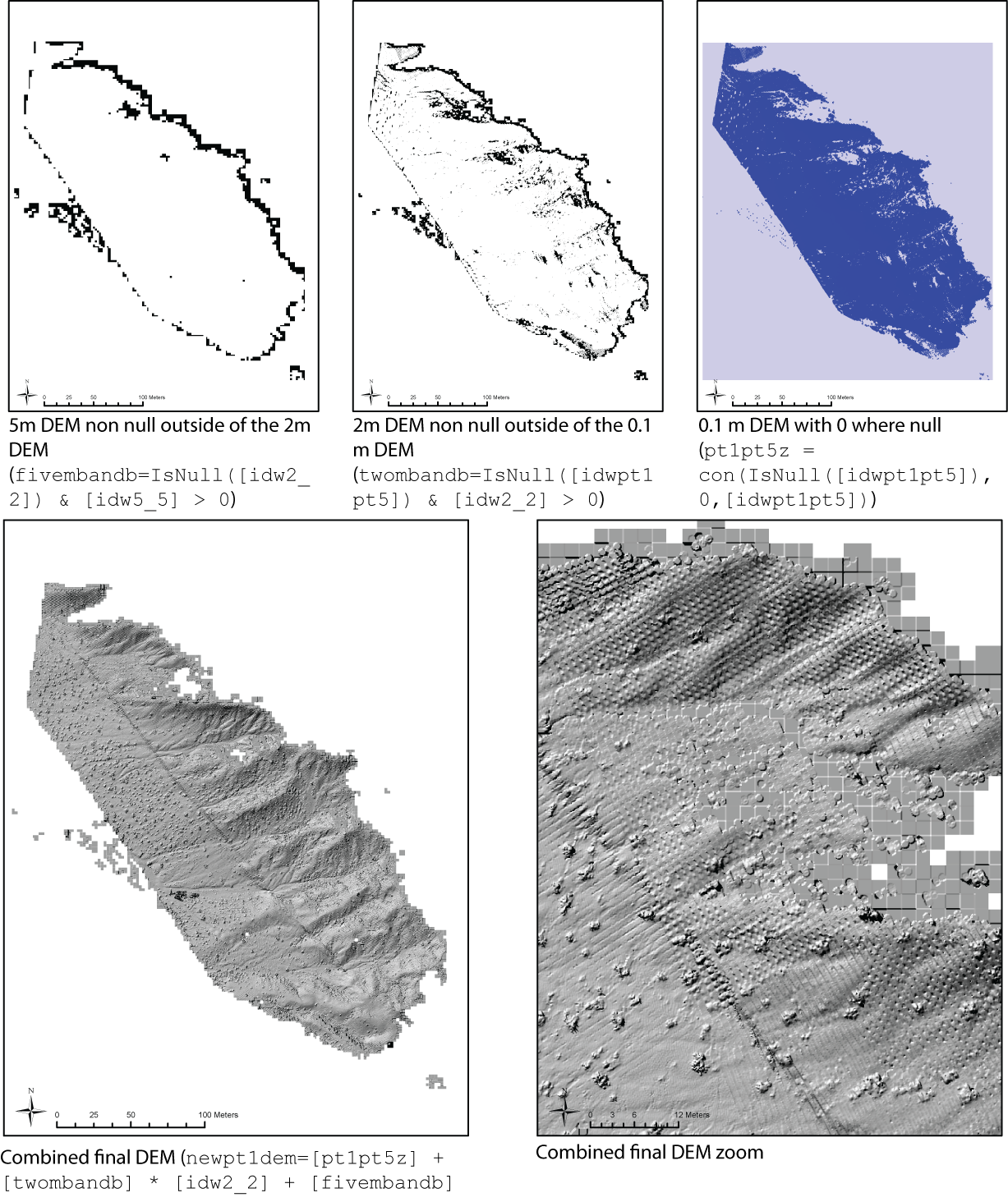
Figure 12. Sequence of grids used to produced the combined final DEM. Upper plots show processed elements which were used to control the combination.

Other processing

From within ArcMap, I could barely get the points loaded (9.54 million point 3 column file). I could not compute any surfaces or a TIN.